The Phong illumination model
Introduction
The Phong equation is one of the most famous lighting models used in graphics for many decades. Its invention is previous to the formulation of the BRDF. Although the Phong model doesn’t produce physically realistic effects like the BRDF, it has been used a lot in many applications and it is still widely in use today.
But why? It turns out that the Phong model, produces fake lighting effects that look great. And that’s the first rule about graphics, if it looks good, it is good. Phong equation is also very simple and cheap to compute.
Nowadays, most applications use Phong shading in combination with more complex techniques to generate good looking graphics. The phong equation
The Phong equation is the sum of three different components: Ambient, Diffuse and Specular; that try to produce the result of different light behaviors.
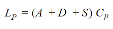
The result of each of this components and, therefore of this equation, is an RGB value that represents the amount of light L (or intensity) in each RGB channel that is reflected at point P in the direction V given the color Cp of the point.
Ambient component
The ambient component represents the light intensity equivalent to indirect lighting. These are the light rays that don’t come directly from a light sources but light bounces around the scene that arrive at the surface of the object.
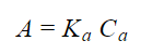
This is just a constant Ka that weights the importance of the ambient component in the equation and Ca is the ambient light color that is a RGB value. The ambient component is the minimum scene light that arrives at the object surface. In this equation, the ambient component is independent of the number or intensity of lights. However, we could calculate K based on the number of lights in the scene to produce a more realistic result.

Diffuse component
The diffuse component represents the light rays that arrive directly from a light source at the surface of the object and spread in multiple and different directions.
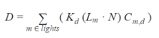
First of all, we have sum over all lights. This means that we have to calculate how each light contributes to the diffuse component of the object and add them together to compute the final diffuse component. Thus, for each light, we calculate the diffuse contribution.
As before, we have a constant Kd that weights the importance of the diffuse component in the equation. Lm is the outgoing light direction, N is the normal vector at point P and Cm,d is the diffuse light color.
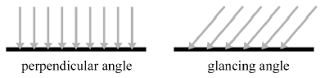
To explain what the dot product does, let’s imagine that the light rays hit a certain surface. If all rays hit the surface with a perpendicular angle (90º degrees) it receives more light than if the angle is glancing. This is called the Lambert cosine law.

Specular component
Finally, the specular component represents the light rays that arrive directly from a light source. Unlike before, these rays are reflected in one specific direction (mirror like).
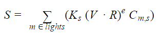
As before, we have to calculate the specular component for each light and then add them. Now we have Ks that weights the importance of the specular component in the equation, V is the outgoing view direction, R is the reflected vector at point P and Cm,s is the specular light color. Here it appears a new parameter (from exponent, but commonly called shininess). This parameter is an exponent of the dot product. But what does the dot product do? In this case, the dot product calculates the angle between the view direction V and the reflected vector R. If the angle is close to 90º, the object is behaving like a mirror so most of the light should be reflected.
The exponent or shininess is useful to tweak how much we want the reflection to be focused in one single point or to be more spread along the surface instead. It is very easy to understand how it works looking at an image: Shininess from 1 to 200 (left to right)
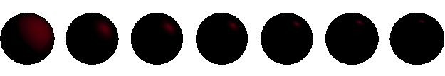
When we use an exponent in a value that ranges from 0 to 1 (not -1 to 1, more on this later), we are making the small values even smaller (ie: 0.1 becomes 0.01) and the higher values don’t get really affected (ie: 0.99 becomes 0.98). Thus, a high shininess means that light rays will be only reflected in that direction where the dot product is really high, or what is the same, that the angle between L and the R is close to 90º.
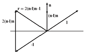
Finally, I think it’s worth mentioning how to calculate the R vector:

It’s quite easy to understand if we take a look at the following image:
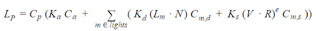
Putting it all together
If we add all the previous equation of the different components, we have the complete Phong equation:
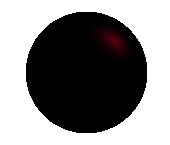
And these are the results of my Ray tracer using the Phong lighting model

Notes
Regarding the Phong coefficients, the ambient is usually the smallest, around 0.1-0.2, while the diffuse and the specular vary between 0.3-0.6.
Usually, the result of the dot product in the formula is clamped to the range [0, 1] from range [-1, 1] using a max(value,0) function . We do this because it doesn’t make sense to have a negative angle. It means that the light is coming from a wrong direction and it shouldn’t be taken into account.
There are some variations to the Phong equation. The most known ones are the Gouraud lighting model and the Blinn-Phong.
The Gouraud lighting model is just the Phong model applied to vertex of a polygon (instead of pixels) and using linear interpolation to calculate the color of the points between the pixels. This tend to produce worst results, but it’s much more cheaper to compute (only once per vertex). It can be easily implemented in the vertex shader using OpenGL.
Blinn-phong is a variation of the Phong equation that is more efficient and the results are almost the same. In some situations, Blinn-phong is even better. The only difference with Phong is that Blinn-Phong, instead of using the reflected vector R to calculate the specular component, it uses the halfway vector H:
This is more efficient than calculating R because it is independent of the view vector V. This means that we can calculate it once at the beginning and then use the same H vector over and over. This may not seem a great improvement, but when working over a million pixels, it is.
References
Fletcher Dunn, Ian Parberry: “3D Math Primer for Graphics and Game Development”
Images generated by my own Raytracer